Algorithms give computers step-by-step instructions to resolve a problem-category in the best possible way.
Asymptotic Notations
- describes the run time of an algorithm based on the input size
Amortized Time
~ Average time taken per function call if the function is called many times
For example, when a Dynamic Array hits the array capacity in it, then it creates a new array with double the size of the old array and copies all the items from old array to the new array. Inserting in ArrayList has two time complexities: O(1), O(n) - since there are 2 time complexities => we use amortized time. So the time complexity of inserting X elements will be
1 + 2 + 4 + 8 + 16 + ... + X = X + X/2 + X/4 + X/8 + ... + 4 + 2 + 1 ~= 2X
So X insertions take about O(2X) time which means the amortized time for each insertion is 2X/X = 2 => O(1)
Space Complexity
Recursive calls takes up stack space (func calls that simultaneously exists in the call stack)
Asymptotic Notations
- describes the run time of an algorithm based on the input size
- Big O: f(N) ∈ O(g(n)) iff there are constants: c, N0 such that f(N) <= c * g(N) for all N0 <= N
- Big Omega: f(N) ∈ Ω(g(n)) iff there are constants: c, N0 such that f(N) >= c * g(N) for all N0 <= N
- Big Theta: f(N) ∈ Θ(g(n)) iff f(N) ∈ O(g(n)) AND f(N) ∈ Ω(g(n))
- -
- Analogy: Electronic Transfer of a file = O(Size of file); Airplane Transfer of a file = O(1)
- -
- Best/Average/Worst case describe the run time of a particular input for that algorithm
- -
- Little O: provides a strict upper-bound (strictly less/faster-than)
- f(N) ∈ o(g(n)) iff there are constants: c, N0 such that f(N) < c * g(N) for all N0 <= N
- Little Omega: provides a strict lower-bound (strictly more/slower-than)
- f(N) ∈ ω(g(n)) iff there are constants: c, N0 such that f(N) > c * g(N) for all N0 <= N
Amortized Time
~ Average time taken per function call if the function is called many times
For example, when a Dynamic Array hits the array capacity in it, then it creates a new array with double the size of the old array and copies all the items from old array to the new array. Inserting in ArrayList has two time complexities: O(1), O(n) - since there are 2 time complexities => we use amortized time. So the time complexity of inserting X elements will be
1 + 2 + 4 + 8 + 16 + ... + X = X + X/2 + X/4 + X/8 + ... + 4 + 2 + 1 ~= 2X
So X insertions take about O(2X) time which means the amortized time for each insertion is 2X/X = 2 => O(1)
Space Complexity
Recursive calls takes up stack space (func calls that simultaneously exists in the call stack)
Recursive Algorithms
Recursion helps reduce the length of the code and makes it easier to read and write.
It uses LIFO structure as each call gets executed from stack.
Tail recursion is when the recursive call is the last thing executed by the function.
*Note: every recursive program can be written iteratively and vice versa is also true.
When analyzing a recursive call's time complexity => draw a tree to see how many recursive calls are made
Recursion uses more memory, because each recursive call (has its own set of variable values) is stored in the stack, and keeps the value there until the call is finished. Stack Overflow occurs when the base case is not reached, and the recursive call is infinitely called and stored in the stack causing the memory to get exhausted.
* Use recursion when you need to:
- compute the nth
- list first n ... items
- compute all ...
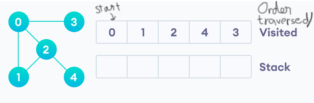
Depth First Search
All nodes have an attribute called 'visited' which is initially set to false. (Or we initialize an empty set called visited and add nodes as we traverse through) Given a starting node of the graph, we mark it visited, and for each child, we traverse through and visit its children.
Time Complexity: O(V + E), Space Complexity: O(V)
|
# DFS algorithm
def dfs(graph, start, visited=None): if visited is None: visited = set() visited.add(start) print(start) for child in graph[start]: if not(child in visited): dfs(graph, child, visited) return visited graph = {'0': set(['1', '2']), '1': set(['0', '3', '4']), '2': set(['0']), '3': set(['1']), '4': set(['2', '3'])} dfs(graph, '0') |
DFS (Iterative)
def dfs(graph, start): stack = [] stack.append(start) visited = set() while (len(stack)) != 0: curr = stack.pop() visited.add(curr) print(curr) children = list(graph[curr]) for i in range(len(children), 0, -1): if not(children[i-1] in visited): #print("stack " + children[i-1]) stack.append(children[i-1]) visited.add(children[i-1]) |
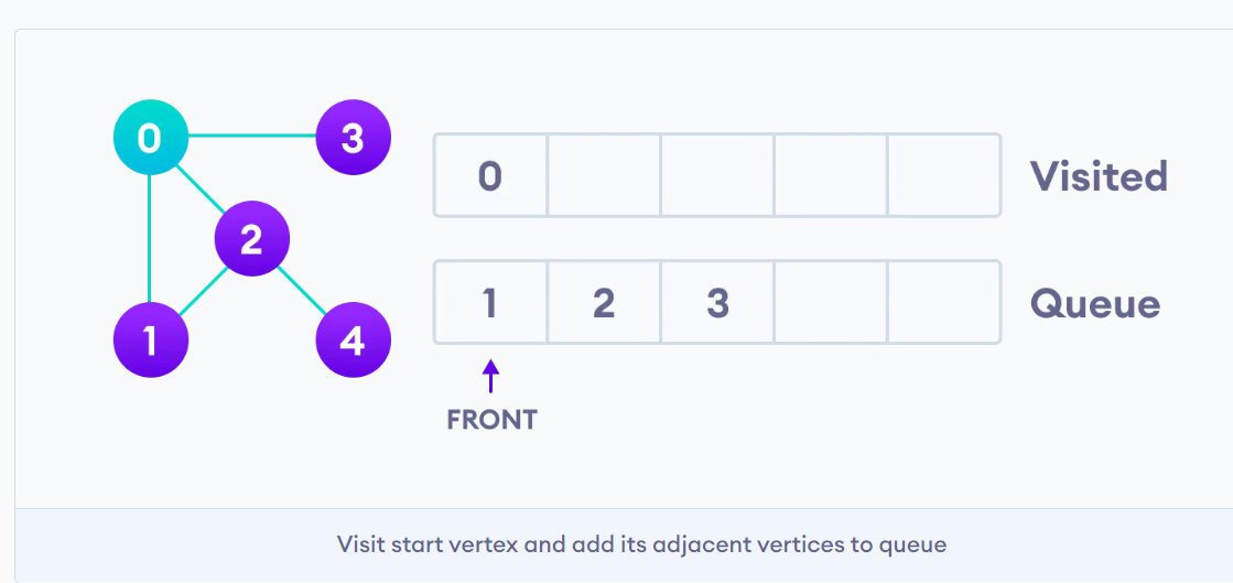
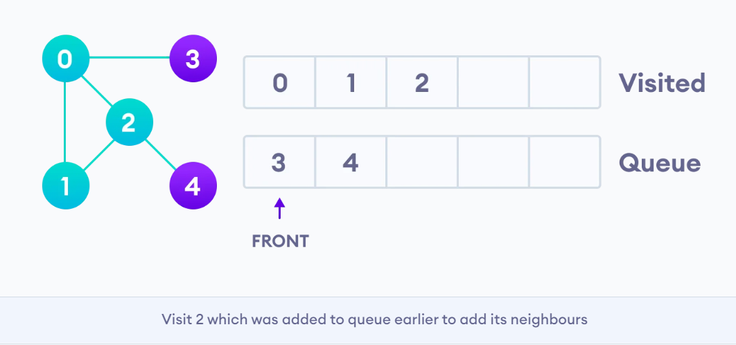
Breadth First Search
Given a starting node of the graph, we mark it visited, and for all of its children, we add them in a queue called 'to-be-visited'. We then visit every node from this queue, while this queue is not empty.
Time Complexity: O(V + E), Space Complexity: O(V)
Given a starting node of the graph, we mark it visited, and for all of its children, we add them in a queue called 'to-be-visited'. We then visit every node from this queue, while this queue is not empty.
Time Complexity: O(V + E), Space Complexity: O(V)
|
# BFS algorithm
def bfs(graph, root): visited = set() queue = [] visited.add(root) print(str(root) + " ", end="") for child in graph[root]: visited.add(child) queue.append(child) while len(queue) != 0: # Dequeue a vertex from queue vertex = queue.pop(0) print(str(vertex) + " ", end="") # If not visited, mark it as visited, and # enqueue it for child in graph[vertex]: if child not in visited: visited.add(child) queue.append(child) if __name__ == '__main__': graph = {0: [1, 2], 1: [2], 2: [3], 3: [1, 2]} print("Following is Breadth First Traversal: ") bfs(graph, 0) |
BFS Traversal
BFS Recursive
def bfs(graph, start, visited=[], rec=set()): if (len(visited) == 0 and start is None) or start in rec: return visited = [start] + visited rec.add(start) if len(visited) != 0: print(visited.pop(0)) for child in graph[start]: if not(child in rec): visited.append(child) rec.add(child) if len(visited) != 0: start = visited.pop(0) rec.remove(start) bfs(graph, start, visited, rec) else: return 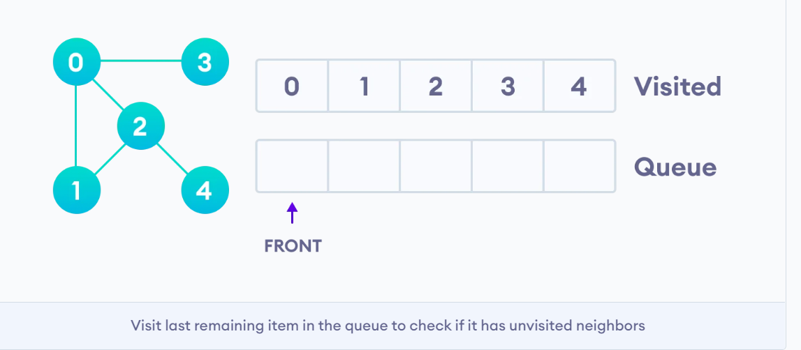
|
Tower of Hanoi
Given: 3 pegs (src, dest, aux), n disks
- move n disks from src to dest peg in min # of moves = (2^n) - 1
- only top disk can be moved
- bigger disk cannot be placed on smaller disk (nth disk cannot be placed on any disk less than n)
Food for Thought on Solution
- In order to solve this problem, we need to first think about base case
If there is only 1 disk, then we move from src peg to dest peg
- If there are 2 disks, then
Step 1: move top disk from src onto aux peg
Step 2: move the last disk from src onto dest peg
Step 3: move that top disk from aux onto dest peg
Time Complexity: O(2^n), Space Complexity: O(1)
|
# Recursive Python function to solve tower of hanoi
def hanoi(n , src, dest, aux): if n == 1: print("Move disk 1 from "+src+ " to "+dest) else: hanoi(n-1, src, aux, dest) print("Move disk "+ n +" from " +src+" to "+dest) hanoi(n-1, aux, dest, src) # Driver code n = 4 TowerOfHanoi(n, 'A', 'C', 'B') # A, C, B are the name of rods |

|
|
GCD (Greatest Common Divisor)
Problem: Greatest possible integer that divides both numbers: a, b When working on a recursion problem, it is important to understand the base case(s) 1) if either a or b equal 0 => return a+b (* if a=0 then return b and if b=0 then return a, but if both equal 0 then return 0) 2) if a and b are equal => return a 3) if a > b: return gcd(a%b, b) else: return gcd(a, b%a) * It is important to note that: a%b (which is remainder of division a/b) will never equal b and vice versa - if a%b equals 0, then the function returns b (since b divides a and itself) and vice versa for b%a - if a%b does not equal 0, then we need to find the greatest common divisor of the remainder and divisor Time Complexity: O(log(min(a, b))), Space Complexity: O(1) |
def gcf(a, b):
if a == 0 or b == 0: return a + b elif a == b: return a elif a > b: return gcf(a%b, b) else: return gcf(a, b%a) |
Divide and Conquer Algorithms
|
- Similar to recursion, divide and conquer breaks down a problem until it's simple enough to resolve it.
- DAC should not be used when the same subproblem occurs many times (ie: for computing Fibonacci => Dynamic Programming should be used). - Overall, DAC reduces time complexity. |

|
Binary Search
The list needs to be already sorted. The recursive method of Binary Search utilizes DAC.
Given: a number/char, a sorted list of items => Find the index where the element is located
The list needs to be already sorted. The recursive method of Binary Search utilizes DAC.
Given: a number/char, a sorted list of items => Find the index where the element is located
Time Complexity: O(log(n)), Space Complexity: O(1)
def binarySearch(array, x, low, high):
if high >= low:
mid = low + (high - low)//2
# If found at mid, then return it, if not => we break the list into 2 halves
if array[mid] == x:
return mid
# Search the left half
elif array[mid] > x:
return binarySearch(array, x, low, mid-1)
# Search the right half
else:
return binarySearch(array, x, mid + 1, high)
else:
return -1 # if elements is not found
Merge Sort
The MergeSort function repeatedly divides the array into two halves until we reach a stage where we try to perform MergeSort on a subarray of size 1.
Time Complexity: O(n*log(n)), Space Complexity: O(n)
Step 1: Divide the given array into 2 halves
# But first check for empty list
if len(array) == 0:
return array
m = len(array) // 2
L = array[:m]
R = array[m:]
Step 2: Make sure both these halves of the array are sorted
mergeSort(L)
mergeSort(R)
Step 3: Merge these 2 sorted arrays
i = j = k = 0
# Until we reach either end of either L or M, pick smaller among elements from L and M and place them in the correct position at A[0..r]
while i < len(L) and j < len(R):
if L[i] < R[j]:
array[k] = L[i]
i += 1
else:
array[k] = R[j]
j += 1
k += 1
# When we run out of elements in either L or M,
# pick up the remaining elements and put in A[r..]
while i < len(L):
array[k] = L[i]
i += 1
k += 1
while j < len(R):
array[k] = R[j]
j += 1
k += 1
Quicksort
Quicksort uses the right most element as pivot, and the remaining elements are partitioned based whether it's smaller or bigger than the pivot element. These partitioned elements are placed on the left and the right side of the pivot element in the array. After that, quicksort is performed on the 2 partitioned sides.
- Quicksort is used when the given array is guaranteed to be non-sorted and space is restricted
Time Complexity: (Worst) O(n^2) (Average)O(n*log n), Space Complexity: O(log n)
Step 1: Check if list is empty - in our case, low and high will indicate this
def quickSort(array, low, high):
if low < high:
Step 2: Call partition to get index of where pivot element is placed
# find pivot element such that
# element smaller than pivot are on the left
# element greater than pivot are on the right
piv = partition(array, low, high)
Step 3: Make sure the elements on the left side of pivot and right side of pivot are sorted
# recursive call on the left of pivot
quickSort(array, low, piv - 1)
# recursive call on the right of pivot
quickSort(array, piv + 1, high)
Step 4: Now Let's implement the partition function
def partition(array, low, high):
Step 5: Choose pivot element
pivot = array[high]
Step 6: Initialize a pointer to keep track of where pivot element should be placed
i = low - 1
Step 7: Every element in the array is compared with the pivot - if an element is smaller than the pivot , then the element is placed at pointer i, or else if element is bigger than the pivot, no action is taken => so all elements smaller than the pivot are placed before pointer i and the big ones after.
# traverse through all elements and compare each element with pivot
for j in range(low, high):
if array[j] <= pivot:
# if element smaller than pivot is found swap it with the greater element pointed by i
i = i + 1
# swapping element at i with element at j
(array[i], array[j]) = (array[j], array[i])
Step 8: Swap the pivot element with the greater element specified by the element after i and return i + 1
(array[i + 1], array[high]) = (array[high], array[i + 1])
return i + 1
MergeSort vs. QuickSort
MergeSort
- it is parallelizable
- works better with linked list
- external sorting requirements (sorting large datasets that don't fit in memory), Merge Sort is often used
- preserves the original order of equal value elements that quicksort does not
QuickSort
- average-case runtime is faster than mergesort
- better cache performance due to its localized and sequential memory access pattern during partitioning
- partitioning process has a lower overhead compared to merging process
Median Finding Algorithm
Given an array A = [1,...,n] of n numbers and an index i, where 1 ≤ i ≤ n, find the ith smallest element of A.
Time Complexity: O(n), Space Complexity: -
# Step 1: i represents the ith smallest element, but if we're finding median, then i = n/2
def median_of_medians(A, i):
# Step 2: Divide the list A into sublists of length 5 and collect the medians of each sublist
sublists = [A[j:j+5] for j in range(0, len(A), 5)]
medians = [sorted(sublist)[len(sublist)/2] for sublist in sublists]
# Step 3: Pivot is the median of the medians
if len(medians) <= 5:
pivot = sorted(medians)[len(medians)/2]
else:
#the pivot is the median of the medians
pivot = median_of_medians(medians, len(medians)/2)
# (Partition) Step 4: Store all elements lower than median of medians (pivot) in low array and the higher ones in high array
low = [j for j in A if j < pivot]
high = [j for j in A if j > pivot]
# Step 5: To get the ith smallest element, we need to check if i is less than n/2 or greater. - This step gets repeated until the median (n/2) = i of array A => so we return median element only when it represents the ith smallest element of array
k = len(low)
if i < k:
return median_of_medians(low,i)
elif i > k:
return median_of_medians(high,i-k-1)
else: #pivot = k
return pivot
Strassen's Matrix Multiplication
The naive way to perform matrix multiplication, where A and B are square NxN matrices has Time Complexity: O(N^3)
def multiply(A, B, C):
for i in range(N):
for j in range( N):
C[i][j] = 0
for k in range(N):
C[i][j] += A[i][k]*B[k][j]
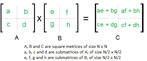
Now we will try using Divide-And-Conquer: we divide the matrix into 4 sub-matrix of N/2 x N/2 and try to solve them recursively. The below image shows how we can go about it.
The naive way to perform matrix multiplication, where A and B are square NxN matrices has Time Complexity: O(N^3)
def multiply(A, B, C):
for i in range(N):
for j in range( N):
C[i][j] = 0
for k in range(N):
C[i][j] += A[i][k]*B[k][j]
Now we will try using Divide-And-Conquer: we divide the matrix into 4 sub-matrix of N/2 x N/2 and try to solve them recursively. The below image shows how we can go about it.
|
However, even in this method, the time complexity is still O(N^3) because there are a total of 8 (N/2) matrix multiplications and 4 additions. Each matrix addition has a time complexity of O(N^2)., so this results in:
T(N) = 8T(N/2) + O(N^2) From Master's Theorem, time complexity of above method is O(N^3) which is the same as the naive method. |
|
Now, if we follow Strassen's formula, we get
Time Complexity ~= O(N^2.8), Space Complexity: O(logn) because instead of performing 8 multiplications after breaking the matrix into 4 sub-matrix, Strassen's only performs 7 sub-matrix multiplication. The below image shows the rule we follow to implement Strassen's Matrix Multiplication algorithm. |

|
import numpy as np
# Step 1: implement the split function, that splits agiven matrix into 4 sub-matrix
def split(matrix):
row, col = matrix.shape
row2, col2 = row//2, col//2
return matrix[:row2, :col2], matrix[:row2, col2:], matrix[row2:, :col2], matrix[row2:, col2:]
# Step 2: Implement Strassen function and the base case when size of matrices is 1x1
def strassen(x, y):
# Base case
if len(x) == 1:
return x * y
# Step 3: Call split function and split each matrix into 4 sub-matrix
a, b, c, d = split(x)
e, f, g, h = split(y)
# Step 4: Compute the 7 matrix multiplication by recursion that are mentioned in Strassen's formula
p1 = strassen(a, f - h)
p2 = strassen(a + b, h)
p3 = strassen(c + d, e)
p4 = strassen(d, g - e)
p5 = strassen(a + d, e + h)
p6 = strassen(b - d, g + h)
p7 = strassen(a - c, e + f)
# Step 5: Perform the required matrix addition mentioned in Strassen's formula
c11 = p5 + p4 - p2 + p6
c12 = p1 + p2
c21 = p3 + p4
c22 = p1 + p5 - p3 - p7
# Step 6: combining the 4 quadrants into a single matrix by stacking horizontally and vertically and return the resulting matrix
c = np.vstack((np.hstack((c11, c12)), np.hstack((c21, c22))))
return c
Karatsuba Algorithm
Even though multiplying small numbers can be considered to be performing in O(1) time, multiplying really large numbers occurs on O(n^2). However, the Karatsuba algorithm can be used to perform multiplication in O(n^1.585). First we will take a look into how the naive method of multiplication is implemented
- Divide each number into 2 halves (for ex: x = 1234 => xH = 12 and xL =34), b = base, in this case it's 10, n = # of digits, in this case it's 4
x = (xH) * (b^(n/2)) + xL, y = (yH) * (b^(n/2)) + yL
- And if we are multiplying x and y together, we get 4 terms to multiply
xy = ((xH) * (b^(n/2)) + xL) * ((yH) * (b^(n/2)) + yL)
= [(xH) * (yH) * (b^n)] + [(xH) * (yL) + (xL) * (yH)] * (b^(n/2)) + (xL * yL)
- For example, if we are multiplying 1234 and 5678, then we get
= (12 * 87 * (10^4)) + ((12 * 65) + (34 * 87)) * (10^(n/2)) + (65 * 34)
- However, if we use Karatsuba's algorithm, we would only need to perform 3 multiplications
a = xH * yH
d = xL * yL
e = (xH + xL) * (yH + yL) - a - d
xy = (a * (b^n)) + (e * (b^(n/2))) + d
Time Complexity: O(n ^ 1.585), Space Complexity: O(n)
# Step 1: Import the required libraries and implement the base case
from math import ceil, floor
def karatsuba(x,y):
if x < 10 and y < 10: # in other words, if x and y are single digits
return x*y
# Step 2: Calculate xH, xL and yH, yL
n = max(len(str(x)), len(str(y)))
m = ceil(n/2) #Cast n into a float because n might lie outside the representable range of integers.
x_H = floor(x / 10**m)
x_L = x % (10**m)
y_H = floor(y / 10**m)
y_L = y % (10**m)
# Step 3: Use recursion to perform the 3 multiplication according to Karatsuba's formula
a = karatsuba(x_H,y_H)
d = karatsuba(x_L,y_L)
e = karatsuba(x_H + x_L, y_H + y_L) - a - d
# Step 4: Perfrorm the final addition and return the result
return int(a*(10**(m*2)) + e*(10**m) + d)
Maximum Subarray Sum
Find the sum of contiguous subarray of numbers which has the largest sum
Time Complexity: O(n * log n), Space Complexity: O(1)
def maxSubArraySum(arr, l, h):
if (l > h):
return 0 # If empty array is not allowed, return -INF
# Base Case: Only one element
if (l == h):
return max(0, arr[l])
m = (l + h) // 2
return max(maxSubArraySum(arr, l, m-1),
maxSubArraySum(arr, m+1, h),
maxCrossingSum(arr, l, m, h))
# Find the maximum possible sum in arr[] auch that arr[m] is part of it
def maxCrossingSum(arr, l, m, h):
# Include elements on left of mid
sm = 0
left_sum = 0
for i in range(m, l-1, -1):
sm = sm + arr[i]
if (sm > left_sum):
left_sum = sm
# Include elements on right of mid
sm = 0
right_sum = 0
for i in range(m, h):
sm = sm + arr[i]
if (sm > right_sum):
right_sum = sm
return max(left_sum + right_sum - arr[m], left_sum, right_sum)
MaxMin DAC
Given an array find the max and min. Naive method would perform 2*(n-1) comparisons but DAC takes (3*n/2)-2 comparisons
def MaxMinDAC (arr, low, high):
if low == high:
return arr[low], arr[low]
elif high - low == 1:
return max(arr[low], arr[high]), min(arr[low], arr[high])
else:
mid = (low + high)//2
L_max, L_min = MaxMinDAC (arr, low, mid)
R_max, R_min = MaxMinDAC (arr, mid+1, high)
return max(L_max, R_max), min(L_min, R_min)
Stock Buy & Sell Profit
Calculate the maximum difference such that the larger element appears after the smaller element.
Time Complexity: O(n), Space Complexity:-
def DivideAndConquerSingleSellProfit(arr):
# Base case: If the array has zero or one elements in it, the maximum profit is 0.
if len(arr) <= 1:
return 0;
# Cut the array into two roughly equal pieces.
left = arr[ : len(arr) / 2]
right = arr[len(arr) / 2 : ]
# Find the values for buying and selling purely in the left or purely in the right.
leftBest = DivideAndConquerSingleSellProfit(left)
rightBest = DivideAndConquerSingleSellProfit(right)
# Compute the best profit for buying in the left and selling in the right.
crossBest = max(right) - min(left)
# Return the best of the three
return max(leftBest, rightBest, crossBest)
Convert Sorted Array to Binary Search Tree
Time Complexity: O(n), Space Complexity:-
# Definition for a binary tree node.
class TreeNode:
def __init__(self, val=0, left=None, right=None):
self.val = val
self.left = left
self.right = right
class Solution:
def sortedArrayToBST(self, nums: List[int]) -> Optional[TreeNode]:
if len(nums) == 0:
return
mid = len(nums)//2
root = TreeNode(val=nums[mid])
root.left = self.sortedArrayToBST(nums[:mid])
root.right = self.sortedArrayToBST(nums[mid+1:])
return root
Construct Binary Search Tree from Preorder Traversal
# Definition for a binary tree node
class TreeNode:
def __init__(self, val=0, left=None, right=None):
self.val = val
self.left = left
self.right = right
class Solution:
def bstFromPreorder(self, preorder: List[int]) -> Optional[TreeNode]:
if len(preorder) == 0:
return None
node = preorder.pop(0)
root = TreeNode(node)
l = []
r = []
for val in preorder:
if val < node:
l.append(val)
else:
r.append(val)
root.left = self.bstFromPreorder(l)
root.right = self.bstFromPreorder(r)
return root
Reverse String
Write a function that reverses a string. The input string is given as an array of characters s
Time Complexity: O(n/2), Space Complexity:-
def reverseString(self, s: List[str]) -> None:
# Modify s in-place, space complexity: O(1)
low = 0
high = len(s)-1
while low < high:
s[low], s[high] = s[high], s[low]
low += 1
high -= 1
Two Sum II - Input Array Is Sorted
Given an array of integers numbers that is already sorted in non-decreasing order, find two numbers such that they add up to a specific target number
Time Complexity: O(n), Space Complexity:-
def twoSum(self, numbers: List[int], target: int) -> List[int]:
# base case: there's exactly one pair that sums to target
if len(numbers) == 2:
return [0, 1]
low = 0
high = len(numbers) - 1
while high > low:
if numbers[low] + numbers[high] == target:
return [low, high]
elif numbers[low] + numbers[high] < target:
low += 1
elif numbers[low] + numbers[high] > target:
high -= 1
Extras & Sorting Algos
Swapping w/o temp var
Swap value of 2 variables without temporary variable
Swap value of 2 variables without temporary variable
- (*using addition)
- a = a + b
- b = a - b # => (a + b) - b
- a = a - b # => (a + b) - a
- (*using xor)
- x = x ^ y
- y = x ^ y
- x = x ^ y
Prime Numbers
Checking for prime numbers
- In order to check if a given number, n is prime,
x You don't need to check if n can be divided by any num from 2 to n-1
o You just need to check if n can be divided by any num from 2 to sqrt(n)
- because for every a * b = n => a <= sqrt(n) and b >= sqrt(n)
Generating a List of Primes: The Sieve of Eratosthenes
* All non-prime numbers are divisible by a prime number
* Given a num n, create a list with size n+1 and set their values as true except for 0 and 1 which will be set to false
* For each number in the list (ie: 2) set false for all numbers that are divisible by 2 except for 2 itself
- repeat this for the next number w/ true value until max is reached
=> final result gives the list of primes from 2 to max
Implementation of Sieve of eratosthenes
def listPrimes(n):
lst = []
for i in range(n+1):
if i == 0 or i == 1:
lst.append(False)
else:
lst.append(True)
i = 2
j = 3
nxt = n+1
while i < (n+1):
for j in range(i+1, n+1):
if i != j and j % i == 0:
lst[j] = False
else:
if nxt > j:
nxt = j
i = nxt
nxt = n+1
for k in range(len(lst)):
if lst[k]:
print(k)
lst = []
for i in range(n+1):
if i == 0 or i == 1:
lst.append(False)
else:
lst.append(True)
i = 2
j = 3
nxt = n+1
while i < (n+1):
for j in range(i+1, n+1):
if i != j and j % i == 0:
lst[j] = False
else:
if nxt > j:
nxt = j
i = nxt
nxt = n+1
for k in range(len(lst)):
if lst[k]:
print(k)
Heap Sort
Given an array, construct a heap tree (parent node is greater than its child nodes in max heap) - Keep popping root elements from heap tree and change the last values of the array
Con: slow on small data sets
Time Complexity: O(n*logn), Space Complexity: O(1)
"""
Args: an array, size of heap (n), and index i.
It compares the value at index i with its left and right children, and if necessary, swaps elements to maintain the max heap property.
"""
def heapify(arr, n, i):
largest = i
left_child = 2 * i + 1
right_child = 2 * i + 2
if left_child < n and arr[left_child] > arr[largest]:
largest = left_child
if right_child < n and arr[right_child] > arr[largest]:
largest = right_child
if largest != i:
arr[i], arr[largest] = arr[largest], arr[i]
heapify(arr, n, largest)
def heap_sort(arr):
n = len(arr)
# Build a max heap - Start from the last non-leaf node and heapify as the indices go up
for i in range(n // 2 - 1, -1, -1):
heapify(arr, n, i)
# Extract elements from the heap one by one
for i in range(n - 1, 0, -1):
arr[0], arr[i] = arr[i], arr[0] # Swap the root with the last element
heapify(arr, i, 0) # Heapify the reduced heap
|
Bubble Sort
Repeated swaps the adjacent elements if they are in the wrong order. 1st iteration and continues until nth iteration ( 5 1 4 2 8 ) –> ( 1 5 4 2 8 ) ( 1 5 4 2 8 ) –> ( 1 4 5 2 8 ) ( 1 4 5 2 8 ) –> ( 1 4 2 5 8 ) ( 1 4 2 5 8 ) –> ( 1 4 2 5 8 ) Time Complexity: O(n^2), Space Complexity: O(1) def bubbleSort(arr): n = len(arr) for i in range(n): # Last i elements are already in place for j in range(0, n-i-1): if arr[j] > arr[j+1]: arr[j], arr[j+1] = arr[j+1], arr[j] |
Why Bubble sort is awful? O(n^2) even on average case performs too many swaps/writes O(n^2) on partially sorted list Pro: w/ Parallel processing => BubbleSort sorts in O(n) time better than Insertion and Selection sorts |
Insertion Sort
The array is split into a sorted and an unsorted part. Values from the unsorted part are picked and placed at the correct position in the sorted part.
Pro: good for partially sorted lists
For example: arr = [12, 11, 13, 5, 6]
[12, 11, 13, 5, 6] => [11, 12, 13, 5, 6] - 1st iter: compare 1st and second element
[11, 12, 13, 5, 6] => [11, 12, 13, 5, 6] - 2nd iter: compare 13 with the last element of the sorted part
[11, 12, 13, 5, 6] => [11, 12, 5, 13, 6] => [11, 5, 12, 13, 6] => [5, 11, 12, 13, 6] - 3rd iter: keep swapping 5 until it is in the correct place
[5, 11, 12, 13, 6] => [5, 11, 12, 6, 13] => [5, 11, 6, 12, 13] => [5, 6, 11, 12, 13] - 4th iter: keep swapping 6 until it is in the correct place
Time Complexity: O(n^2), Space Complexity: O(1)
def insertionSort(arr):
for i in range(1, len(arr)):
key = arr[i]
# Keep swapping curr element(key) in the sorted section until curr element is put in the correct place
j = i-1
while j >= 0 and key < arr[j] :
arr[j + 1] = arr[j]
j -= 1
arr[j + 1] = key
Shell Sort
1. Choose a gap (usually: g = len(lst)//2 and the gap keeps dividing itself by 2 until it reaches 1)
2. Insertion Sort with Gaps: For each gap value, Shell Sort performs an insertion sort on the elements that are "gap" positions apart.
3. In the final pass with a gap of 1, Shell Sort behaves like a regular Insertion Sort, but the elements are now partially sorted due to the previous passes.
Time Complexity: O(n^2) ~ depending on gap sequence; on average better than n^2, Space Complexity: O(1)
|
def shell_sort(arr):
n = len(arr) gap = n // 2 # Initial gap value while gap > 0: for i in range(gap, n): temp = arr[i] j = i while j >= gap and arr[j - gap] > temp: arr[j] = arr[j - gap] j -= gap arr[j] = temp gap //= 2 # Reduce the gap # Example usage arr = [12, 34, 54, 2, 3] shell_sort(arr) print("Sorted array:", arr) |
|
Selection Sort
In each iteration, the minimum element from the unsorted part is swapped with the end of the sorted part.
Pro: Minimized Swaps
For example: arr = [64, 25, 12, 22, 11]
[64, 25, 12, 22, 11] => [11, 25, 12, 22, 64] - 1st iter: Swap 11 (smallest element) with end of sorted part 64
[11, 25, 12, 22, 64] => [11, 12, 25, 22, 64] - 2nd iter: Swap 12 (next smallest element) with end of sorted part 25
[11, 12, 25, 22, 64] => [11, 12, 22, 25, 64] - 3rd iter: Swap 22 (next smallest element) with end of sorted part 25
[11, 12, 22, 25, 64] => [11, 12, 22, 25, 64] - 4th iter: Swap 25 (next smallest element) with end of sorted part 25
[11, 12, 22, 25, 64] => [11, 12, 22, 25, 64] - 5th iter: Swap 64 (next smallest element) with end of sorted part 64
Time Complexity: O(n^2), Space Complexity: O(1)
import sys
A = [64, 25, 12, 22, 11]
for i in range(len(A)):
# Find the minimum element from the unsorted part
min_idx = i
for j in range(i+1, len(A)):
if A[min_idx] > A[j]:
min_idx = j
# Swap the found minimum element with end of sorted part
A[i], A[min_idx] = A[min_idx], A[i]
Topological Sort
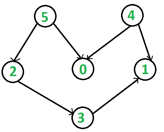
Topological sort (only works for Directed Acyclic Graph) is a linear ordering of vertices such that for every directed edge u->v, vertex u comes before v in the ordering.
Topological sort (only works for Directed Acyclic Graph) is a linear ordering of vertices such that for every directed edge u->v, vertex u comes before v in the ordering.
|
For example, given a set of courses with prerequisites, topo sort will give you an order in which you can take all the courses
Right side shows a DAG. The following are topological sort of the given graph:
Time Complexity: O(V + E), Space Complexity: O(V) |
|
from collections import defaultdict
class Graph:
def __init__(self, vertices):
self.graph = defaultdict(list) # dictionary containing adjacency List
self.V = vertices # No. of vertices
def addEdge(self, u, v):
self.graph[u].append(v)
# helper function
def topologicalSortUtil(self, v, visited, stack):
visited[v] = True
# Recur for all the vertices adjacent to this vertex
for i in self.graph[v]:
if visited[i] == False:
self.topologicalSortUtil(i, visited, stack)
# Push child vertices before parent
stack.append(v)
# main function
def topologicalSort(self):
# Initially mark all the vertices as not visited
visited = [False] * self.V
stack = []
# Get all vertices from graph added to stack
for i in range(self.V):
if visited[i] == False:
self.topologicalSortUtil(i, visited, stack)
print(stack[::-1]) # return list in REVERSE order
Bucket Sort
Useful when input is uniformly distributed over a range and for floating point values
Useful when input is uniformly distributed over a range and for floating point values

Time Complexity: O(n) - if all numbers are evenly distributed, (worst case = O(n^2)) Space Complexity: O(1)
def bucketSort(arr):
# Find the range of input values
min_val = min(arr)
max_val = max(arr)
range_val = max_val - min_val + 1
buckets = []
num_buckets = len(arr) # Determine the number of buckets
for i in range(num_buckets):
buckets.append([])
# Distribute input values into different buckets
for num in arr:
index = int((num - min_val) / range_val * (num_buckets - 1))
buckets[index].append(num)
# Sort each bucket and concatenate them
sorted_arr = []
for bucket in buckets:
sorted_bucket = sorted(bucket)
sorted_arr.extend(sorted_bucket)
return sorted_arr
|
Radix & Counting Sort
Sorts numbers based on digits of the same place value and uses counting sort as a subroutine. It is used when the numbers are in large ranges Time Complexity: O(n+k) Space Complexity: O(max # of digits) ~ same as counting sort |

|
|
# Counting sort according to digit represented by exp
def countingSort(arr, exp1): n = len(arr) # Will have the final sorted arr output = [0] * (n) # initialize count array count = [0] * (10) # Store count of occurrences for i in range(0, n): index = arr[i] // exp1 count[index % 10] += 1 # Change count to contains actual position of this digit in output array for i in range(1, 10): count[i] += count[i - 1] # Build the output array i = n - 1 while i >= 0: index = arr[i] // exp1 output[count[index % 10] - 1] = arr[i] count[index % 10] -= 1 i -= 1 # Copying the output array to arr[] i = 0 for i in range(0, len(arr)): arr[i] = output[i] |
|
def radixSort(arr):
# Find max num to know number of digits
max1 = max(arr)
# Do counting sort for every place value. *Note exp is 10^i where i is current digit number
exp = 1
while max1 / exp >= 1:
countingSort(arr, exp)
exp *= 10
# Find max num to know number of digits
max1 = max(arr)
# Do counting sort for every place value. *Note exp is 10^i where i is current digit number
exp = 1
while max1 / exp >= 1:
countingSort(arr, exp)
exp *= 10
- Closest Pair of Points
- Fast Fourrier Transform
- Convex Hull