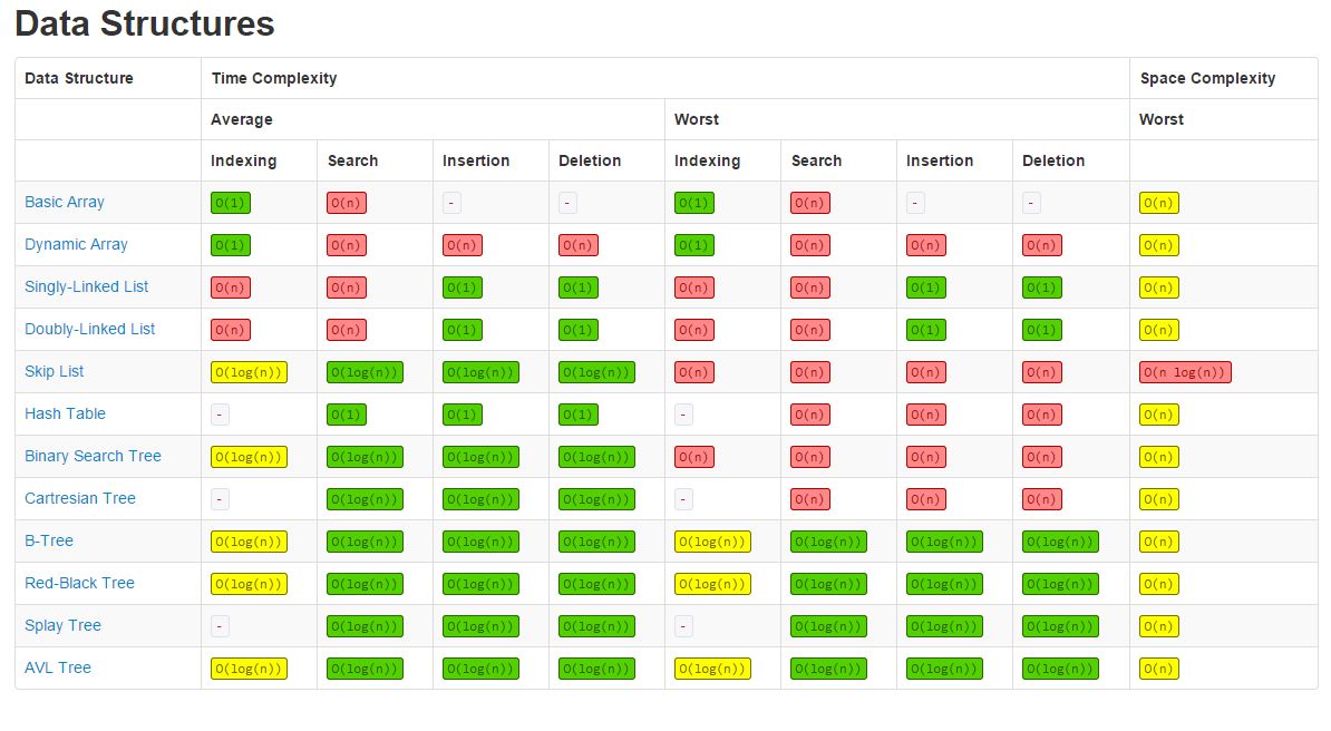
Data Structures

Data Structures are how the computer stores and organizes data. Data Structures help manage large amounts of data efficiently for uses such as large databases, general files stored in the computer, and internet indexing services. It is used based on its ability to fetch and store data at any place.

Primitive Data Structure: It is a predefined way of storing data in the system and all sets of operations are also pre-defined. ex: char data structure consists of a-z, A-Z, and some other symbols.

Non-primitive Data Structure: It can store any set of values that the user wants to store. There are 2 types

Linear Data Structure: Elements are arranged sequentially
- Arrays: collection of items stored at contiguous memory locations
- Stacks: follows the LIFO (Last In, First Out) principle
- Queues: follows the FIFO (First In, First Out) principle
- Linked List: a dynamic data structure where the number of nodes in the list is not fixed and can grow/shrink

Non-Linear Data Structure: data elements can be attached to more than 1 elements. It utilizes memory efficiently and does allocate meory in advance
- Trees: hierarchical data structure
- Graphs: pairs of node/vertices are connected by edges

* Arrays are considered static data structures. It allocates contiguous slots of memory and when a new element is inserted, a bigger array is allocated and the elements are copied over to the bigger array. Stacks, queues, trees, and graphs that are implemented using an array will also be static. However, Linked list is a type of dynamic data structure that does not allocate memory when initiated. It is stored in various memory locations and are connected via pointers. Stacks, queues, trees, and graphs that are implemented using a linked lists can be dynamic.

The operation on each dynamic set can be organized into 2 parts:

Query Operations: Helps to get some info about the dynamic set. ex: search(S, k), getMax(S), getMin(S), printSet(S), etc.
Modifying Operations: Helps to update the dynamic set. ex: insert(S, x), delete(S, x), Merge(S1, S2)

Arrays

- It is a data structure of fixed-size, which can hold items of the same data type. Arrays are indexed, meaning that random access is possible.
- Elements in the array are stored at contiguous memory locations

- Inserting and deleting elements from an array takes O(n) time because:
- when inserting an element, first a new array with increased size must be created, then copy the existing elements and add the new element
- for deleting a new array of reduced size is created

- Byte address of element A[i] = base address (address of the first element in the array) + size of data type * (i)

Applications:
- time complexity for access even on worst case is O(1), but everything else is O(n)
- good for storing multiple values in a single variable
- used as the building blocks for other data structures
- can also be used for different sorting algorithms, ie: insertion sort, quick sort, bubble sort, merge sort

LeetCode / CodingInterview implementations of Arrays are posted here

______________________________________________________________________________________

Linked Lists

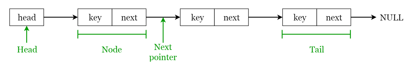
A linked list is a sequential structure that consists of a sequence of items in linear order which are linked to each other. Data can only be accessed sequentially and random access is not possible. However, the number of elements in a linked list is not fixed and can grow and shrink on demand.

Linked List Terms

Elements in a linked list are known as nodes.
Each node contains a key and a pointer to its successor node, known as next.
The attribute named head points to the first element of the linked list.
The last element of the linked list is known as the tail.

Types of Linked Lists

Singly linked list — Traversal of items can be done in the forward direction only.
Doubly linked list — Traversal of items can be done in both forward and backward directions. Nodes consist of an additional pointer known as prev, pointing to the previous node.
Circular linked lists — Linked lists where the prev pointer of the head points to the tail and the next pointer of the tail points to the head.

Linked list operations

Search: Find the first element with the key k in the given linked list by a simple linear search and returns a pointer to this element
Insert: Insert a key to the linked list. An insertion can be done in 3 different ways; insert at the beginning of the list, insert at the end of the list and insert in the middle of the list.
Delete: Removes an element x from a given linked list. You cannot delete a node by a single step. A deletion can be done in 3 different ways; delete from the beginning of the list, delete from the end of the list and delete from the middle of the list.

Applications of linked lists

Used for symbol table management in compiler design.
Used in switching between programs using Alt + Tab (implemented using Circular Linked List).

LeetCode / CodingInterview implementations of Linked Lists are posted here

______________________________________________________________________________________

Stacks & Queues

Stacks
A stack is a LIFO (Last In First Out - the element placed at last can be accessed at first). The following are operations that can be performed on a stack:

Push: Insert an element on to the top of the stack.
Pop: Delete the topmost element and return it.
Peek: Return the top element of the stack without deleting it.
isEmpty: Check if the stack is empty.
isFull: Check if the stack is full.

Applications of stacks

Used for expression evaluation (e.g.: shunting-yard algorithm for parsing and evaluating mathematical expressions).
Used to implement function calls in recursion programming.

LeetCode / CodingInterview implementations of Stacks are posted here

Queues
A queue is a FIFO (First In First Out — the element placed at first can be accessed at first). The following are operations that can be performed on a queue:

Enqueue: Insert an element to the end of the queue.
Dequeue: Delete the element from the beginning of the queue.
isEmpty: Check if the queue is empty.
isFull: Check if the queue is full.

Applications of Queues

Used to manage threads in multithreading.
Used to implement queuing systems (e.g.: priority queues).

LeetCode / CodingInterview implementations of Queues are posted here

______________________________________________________________________________________

Hash Table

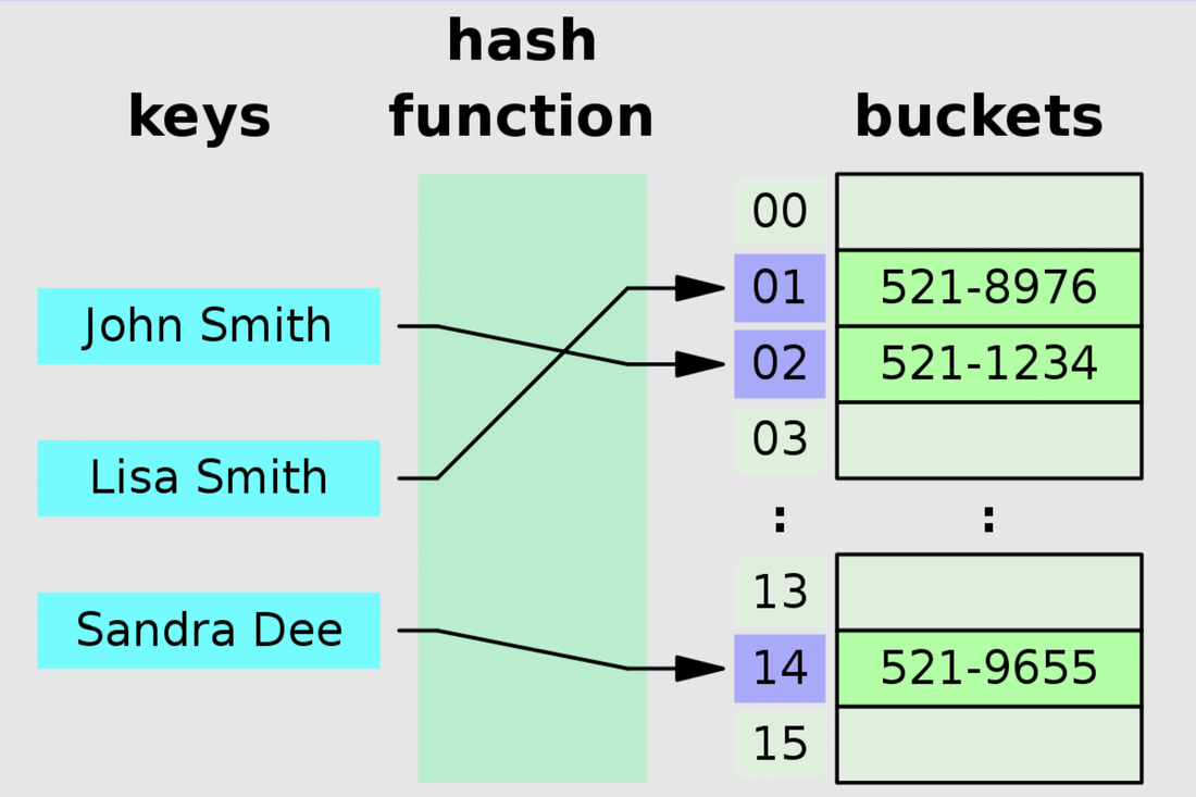
- It is a data structure that stores data in an array format, where each data value has its own unique index value. Access of data becomes very fast if we know the index (where its stored in memory) of the desired data. The Hash Function uses a range of key values into a range of indexes of an array.
For Ex:- (key, value) pairs: (1, 20); (2, 70); (42, 80); (4, 25)
Using the modulo hash function and the size of our hash table is 20
Key Hash Array Index
1 1 % 20 = 1 1
2 2 % 20 = 2 2
42 42 % 20 = 2 2
4 4 % 20 = 4 4

Hash Map Collision - It is when the hash function provides the same index for different key values. If the available space (hash table size is infinite, this can be completely avoided) However, in order to handle this, there are 2 methods:

Separate Chaining: The idea is to make each cell of hash table point to a linked list of records that have the same hash function value Drawbacks
- Wastage of space (some slots of hash table may never get used)
- If the chain becomes too long, then search time can become O(n) in the worst case
- Poor cache performance (since linked list stores in non-contiguous memory locations)

Other methods for chaining include
- if the keys are ordered, then instead of creating a linked list, a balance binary search tree can be implemented => worst-case = O(log n)
- Dynamic Perfect Hashing: 2-level hash tables are used to reduce the look-up complexity, the 2nd hash table will be much bigger in size i^2, so that collisions are less likely to occur => worst-case = O(1)
- Fusion Tree: A type of B-tree that could result in O(1) time for operations with high probability and O(log n) time for others

Open Addressing: All elements are stored in the hash table itself (so size of table must be greater or equal to the number of keys). There are a few ways to do this

Linear Probing: If the slot provided by the hash function is full, then we linearly probe for the next slot.
Let S be the table size, x be any provided key and hash(x) be the hash function that results the index where values can be stored

If slot hash(x) % S is full, then we try (hash(x) + 1) % S
If (hash(x) + 1) % S is also full, then we try (hash(x) + 2) % S
If (hash(x) + 2) % S is also full, then we try (hash(x) + 3) % S and so on ...

Quadratic Probing: We look for the i^2th slot in the ith -iteration

If slot hash(x) % S is full, then we try (hash(x) + 1*1) % S
If (hash(x) + 1*1) % S is also full, then we try (hash(x) + 2*2) % S
If (hash(x) + 2*2) % S is also full, then we try (hash(x) + 3*3) % S and so on ...

Double Hashing: Use another hash function, hash2(x)

If slot hash(x) % S is full, then we try (hash(x) + 1*hash2(x)) % S
If (hash(x) + 1*hash2(x)) % S is also full, then we try (hash(x) + 2*hash2(x)) % S
If (hash(x) + 2*hash2(x)) % S is also full, then we try (hash(x) + 3*hash2(x)) % S and so on ...

Linear probing has the best cache performance but suffers from clustering (too many keys follow the same chaining path). Double hashing has poor cache performance but no clustering and quadratic probing is between the 2.

Some other methods for open addressing include:
- Coalesced Hashing: It is suited for fixed-memory allocation. The collision is resolved by identifying the largest-indexed empty slot on the hash table, and the colliding value is inserted into that slot.
- Cuckoo Hashing: Guarantees O(1) worst-case lookup complexity. It resolves collisions by maintaining 2 hash tables with 2 different hash functions. If procedure enters into infinite loop (noticed from a loop counter) then new hash functions are assigned.
- Hopscotch Hashing: Search in at most H buckets (the hop-range) based on hop-info bitmap. H is a constant.
- Robin Hood Hashing: Collisions are resolved through favouring the displacement of the element that is farthest/ longest probe sequence length from its "home location" (allows for distribution of elements in the hash table)

Basic Syntax of how to use Hashmaps and HashSets in Python and Java

Hash Map Cheat Sheet

To identify a chain in Linked List

- set fast var => x2 speed ----
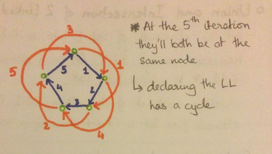
- set slow var => x1 speed ----
- if they are equal => cycle exists
else fast reaches end of linked list => cycle doesn't exist

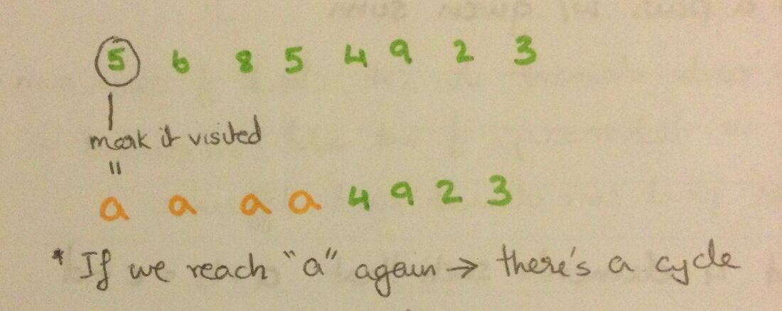
(And) If Linked List may have repeated elements

- leave 'bread crumbs'
- make a copy of LL and change the visited nodes' value

Removing "If" statements => by setting values based on given input

- store expected input values in a dictionary
ex:- {"I":1, "V":5, "X":10, "L":50, "C":100, "D":500, "M":1000}

When you have to keep track of multiple variables/values

- for example, which number occurs most in a list => dictionaries/hashmaps can be used as a counter

Is Isomorphic?

  - check if each element in list A is mapped to exactly 1 element in B & vice versa
  - build a dictionary w/ A elements as keys and B elements as values & vice versa
  - if any element is mapped to more than 1 value => return False else return True

All elements in a given list is unique

=> by creating a hashset >> len(lst) == len(set(lst))

Anagram

ex: - word1 = 'Nathaniel Black' is an anagram of => word2 = 'Annabella Thick'
- make a counter using dictionary for word1
- then check by subtracting for each letter used in word2

Union and Intersection of 2 Linked Lists

  - put the elements of lst1 into a dictionary
  - traverse through lst2, for each element in dictionary => add it to intersection list
  - create a hashset of elements in lst1, then for all elements from lst2 (hashset does not take in duplicates) => union list

Find a pair w/ given sum

  - for each element in lst, check if given_sum - current_element is in dictionary
  if not, then add curr_element in dictionary
  else print curr_element and difference

Find 4 elements such that: a + b = c + d

- store sum of each pair as key, and the pair as its value
- if a sum already exists in the dictionary with different pairs, print the pairs

Missing elements of a range

  - put all elements of the lst into a dictionary
  - loop through the range - if an element is not in the dictionary
  => append it to missing element list

Longest consecutive subsequence

- given a list, put all the elements into a dictionary
- loop through each element - check if curr_element is the starting point by seeing if curr_element-1 is in dictionary
- if curr_element is the starting point, see how long the consecutive subsequence is => store the longest length

Trees

A hierarchical structure where data is organized based on levels and are liked to each other.

Types of Trees:

General Tree / N-ary Tree - Each node can have any (or up to N) number of children
Binary Tree - Each node can have at most 2 children
Binary Search Tree - Left child must value lower than node and right child must have value higher than node
AVL Tree - Self-balancing Binary Search Trees. The balancing factor is the difference in heights between the left and right subtrees, and its values are (-1), 0, and 1.
Red Black Tree - A kind of self-balancing binary search tree where each node stores an extra bit color (red or black)
B-Tree - Self-balancing tree that maintains sorted data
Heaps - parent nodes have the max/min value and its child nodes have lower/higher values
Treap - BST + Heap - each node contains 2 values: keys (following BST property), priority (following Heap property)
Splay Tree. - A BST with an additional property that recently accessed elements are quick to access again

Tree Implementations

Graphs

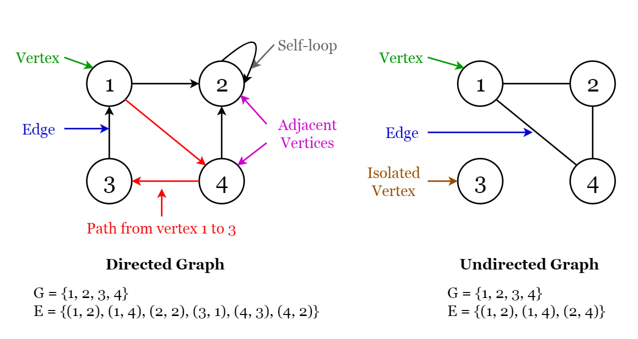
Most graphs are defined as a slight alteration of the following rules:

A graph is made up of two sets called Vertices and Edges
The Verticies are some form of a node type
Each element of the Edge set is a pair consisting of two elements from the Vertices set
Order of a graph = # of vertices in the graph
Size of a graph = # of edges in the graph
2 nodes/vertices are Adjacent => connected by an edge
Self-loop: edge from a vertex to itself
Isolated vertex: no edge connecting to another node

Bridge: An edge whose removal will simply make the graph disconnected
Null graph: A graph is said to be null if there are no edges (but may have isolated vertices)
Cyclic graph: A graph containing a cycle (Opposite is Acyclic/Forest graph)
Weighted graph: Edges that contain a value
Connected graph: Does not have any isolated vertex
Complete graph: Any node can be reached from any node through 1 edge

Some of the types of graphs:

Directed graph: edges have a direction indicating start vertex and end vertex
Undirected graph: edges have no direction

Graphs can be represented through:

Adjacency Matrix - First row and first column of the matrix denotes the vertices. The rest of the cells contains either 0 or1

Adjacency List - An array of linked list. Elements in array contain nodes of the graph and each node is liked to all the nodes it connects to.

Applications of Graphs:

Social media networks
Web pages and links by search engines.
Locations and routes in GPS